Using CoReCon: tutorial

0. Installation

WARNING: CoReCon is still in the beta-testing phase.

CoReCon can be installed as a python module, using:

pip install corecon

and then loaded e.g. using:

import corecon as crc

If you have already installed CoReCon and wish to upgrade it to the latest version, use:

pip install -U corecon

1. Data organization and retrieval

CoReCon stores data in an individual DataEntry class for each data source. The available fields are described in Data Entry Template, while the available utility functions are described below.

Available quantities are listed in the section Available constraints, and can also be retrieved from python using:

available_fields = crc.get_fields()

This returns a tuple containing all available field names (as strings). Most of the fields have synonyms, i.e. alternative names, that can be retrieved using:

field_synonym = crc.get_field_synonyms("quasar_luminosity_function")

These strings (the field name and its synonyms) are used to specify the data to load, using (for e.g. the quasar luminosity function):

qlf = crc.get("quasar_luminosity_function")

The returned object (qlf in the example above) is a custom class derived from python dictionaries. As such, this Field class can be treated as a python dictionary with some additional attributes and functions. For instance, the individual entries can be obtained by a simple query of the dictionary keys, e.g.

for k in qlf.keys():
    print(k)

> Kulkarni et al. 2019
> Giallongo et al. 2015
> McGreer et al. 2013
> Yang et al. 2016
> Willott et al. 2010
> Jiang et al. 2016
> Kashikawa et al. 2015
> Glikman et al. 2011
> Giallongo et al. 2019
> Ross et al. 2013

In addition, it provides descriptors for the physical quantity represented and functions that make easy to manipulate and filter the provided constraints. The class attribute field_description (which is NOT part of the dict keys) contains a string with a breif description (using matplotlib’s Math Text) of the quantity used in values, err_up, err_down, including their units (if present).

print(qlf.field_description)
> ...

It is also possible to retrieve all available constraints using:

all_dicts = crc.get_all_dicts()

which returns a dictionary, whose keys are the available field. Each key is associated to the result of invoking crc.get() with the same key.

Each dictionary entry in a Field class describes a single constraint (i.e. a single scientific publication/dataset), packaged in a DataEntry class. Its attributes can be retrieved simply using e.g.:

values = qlf['McGreer et al. 2013'].values

The available attributes are described in Data Entry Template. In addition, CoReCon automatically creates attributes from the field name and from each one of the dimensions_descriptors, assigning - respectively - the content of the values and the properly-sliced content of the axes attributes. The name of these self-generated attributes is the same as the corresponding field name or dimension descriptor, with spaces replaced by _ and non-alphanumeric characters removed. For instance:

qlf['McGreer et al. 2013'].dimensions_descriptors
> ["redshift", "M 1450"]

qlf['McGreer et al. 2013'].M_1450
> array([-28.05, -27.55, -27.05, -26.55, -26.05, -27, -26.45, -25.9, -25.35, -24.8, -24.25], dtype=object)

Finally, for convenience, additional non-standard attributess are listed in

extra_data = qlf['McGreer et al. 2013'].extra_data

Individual entries can also be directly retrieved using a specific syntax for the argument of the get function, i.e.

single_entry = crc.get('quasar_luminosity_function/McGreer et al. 2013')

In case you want to add your own dataset, this can be done simply adding a properly-formatted file into one of the data/ subdirectories. You can find more information on the format in Data Entry Template. For convenience, such template can be retrieved directly from CoReCon using:

template_string = crc.get_data_entry_template()

which returns the template as a string.

2. Utility functions

CoReCon provides also some basic utilities functions. These are split between the basic module and the Field class.

Available constraints within a redshift range can be retrieved with:

qlf = crc.get("quasar_luminosity_function")
qlf_zrange = qlf.filter_by_redshift_range(6, 7)

Similarly, the data available can be filtered to return only upper or lower limits, using:

qlf_ll = qlf.get_lower_limits()
qlf_ul = qlf.get_upper_limits()

In the same way, the constraints can be filtered based on the value of their extracted keyword, using:

qlf_extracted = crc.filter_by_extracted("qlf", True)

In all these filter functions, the returned object is a copy of the original Field class except for the fact that it only contains the entries satisfying the filtering condition. This allows for easy concatenation, e.g.

qlf = crc.get("quasar_luminosity_function")
qlf_zrange = qlf.filter_by_redshift_range(6, 7)
qlf_zrange_ll = qlf_zrange.get_lower_limits()

See Functions Documentation for a complete list of available filters.

In each DataEntry, upper and lower limits can be swapped (e.g. to be used in derived quantity, for instance 1-ionised_fraction) using:

qlf['Kulkarni et al. 2019'].swap_limits()

CoReCon uses numpy.nan to indicate missing data entries. In case they need to be replaced (e.g. for plotting or operation on data), CoReCon provides the following utility:

qlf['Kulkarni et al. 2019'].nan_to_value('values', 0.0)

where the first argument is a string among ‘values’, ‘err_up’, ‘err_down’, ‘all’ that specify in which DataEntry array NaN should be replaced. The second argument, i. e. the value to replace NaN with, can either be a scalar or an array of the appropriate shape.

Finally, CoReCon provides a function that replaces all the entries in err_up and err_down corresponding to upper or lower limits with a user defined value v, which can be specified as a fraction of the correspondent value entries. It can be used, e. g. to easily set arrow length when plotting limits with matplotlib.pyplot’s errorbar() function. Error on limits can be set using:

qlf['Kulkarni et al. 2019'].set_lim_errors(0.1, frac_of_values=True)

The documentation for CoReCon public functions can be found at Functions Documentation.

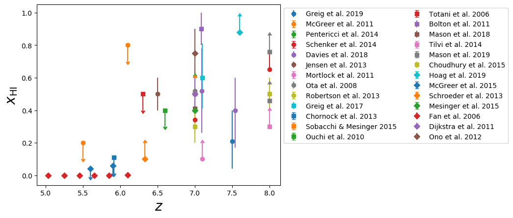
3. Complete example

Finally, we provide here a simple head-to-tail example of usage, namely to create a plot of the ionized fraction evolution with redshift.

import corecon as crc
import matplotlib.pyplot as plt
import numpy as np

#get ionized fraction
ionfr = crc.get("ionized_fraction")

#create figure, ax, and markers cycle
fig, ax = plt.subplots(1)
markers = ['o', 's', 'D', '*']

#loop over available datasets
for ik,k in enumerate(ionfr.keys()):

    #if k=="field_description":
    #    continue

    #find which axes corresponds to redshift
    zdim = np.where(ionfr[k].dimensions_descriptors == "redshift")[0][0]

    #get format
    fmt = "%sC%i"%(markers[ik//10], ik%10)

    #transform to neutral fraction
    ionfr[k].values = 1-ionfr[k].values  #NB: it now contains the neutral fraction!
    # ...need to swap errors
    ionfr[k].swap_errors()
    # ...and limits as well
    ionfr[k].swap_limits()
    #transform NaNs (in errors) into values to set arrow length
    ionfr[k].nan_to_values(['err_up', 'err_down'], 0.1)

    #plot
    ax.errorbar(ionfr[k].axes[:,zdim], ionfr[k].values,
                yerr=[ionfr[k].err_down, ionfr[k].err_up],
                lolims=ionfr[k].lower_lim, uplims=ionfr[k].upper_lim,
                fmt=fmt, label=k)

#move legend to side
ax.legend(bbox_to_anchor=(1.0, 1.0), bbox_transform=ax.transAxes, loc='upper left')

#save figure and close
fig.savefig( "neutral_fraction_evolution.png" , bbox_inches='tight')
plt.close(fig)

The above script produce the following plot: